生存分析别只用Cox回归了,试试机器学习之随机森林生存分析(randomForestSRC)怎么样?
前言
随机生存森林通过训练大量生存树,以表决的形式,从个体树之中加权选举出最终的预测结果。
构建随机生存森林的一般流程为:
Ⅰ. 模型通过“自助法”(Bootstrap)将原始数据以有放回的形式随机抽取样本,建立样本子集,并将每个样本中37%的数据作为袋外数据(Out-of-Bag Data)排除在外;
Ⅱ. 对每一个样本随机选择特征构建其对应的生存树;
Ⅲ. 利用Nelson-Aalen法估计随机生存森林模型的总累积风险;
Ⅳ. 使用袋外数据计算模型准确度。
生存,竞争风险生存设置需要一个时间和审查变量,应该在公式中使用标准生存公式规范作为结果。一个典型的公式是这样的:Surv()~。状态是用户数据集中事件时间和状态变量的变量名。对于生存森林(Ishwaran et al. 2008),审查变量必须编码为一个非负整数,0为审查保留,(通常)1=死亡(事件)。对于竞争风险森林(Ishwaran et al., 2013),实现类似于生存,但有以下注意事项:审查必须编码为非负整数,其中0表示审查,非零值表示不同的事件类型。而0,1,2,…,J为标准,建议事件可以不连续编码,但必须始终使用0进行审查。将拆分规则设置为logrankscore将导致生存分析,其中所有事件都被视为相同类型。通常,竞争风险需要比生存设置更大的节点大小。
软件安装
RandomForestSRC 是美国迈阿密大学的科学家 Hemant Ishwaran和 Udaya B. Kogalur开发的随机森林算法,它涵盖了随机森林的各种模型,包括:连续变量的回归,多元回归,分位数回归,分类,生存性分析等典型应用。RandomForestSRC 用纯 C 语言开发,其主文件有 3 万多行代码,集成在 R 环境中。
if (!require(randomForestSRC)) install.packages("randomForestSRC")
if (!require(survival)) install.packages("survival")

library(randomForestSRC)
library(survival)
数据读取
Veteran’s Administration Lung Cancer Trial Description Randomized trial of two treatment regimens for lung cancer. This is a standard survival analysis data set. Format trt: 1=standard 2=test celltype: 1=squamous, 2=smallcell, 3=adeno, 4=large time: survival time status: censoring status karno: Karnofsky performance score (100=good) diagtime: months from diagnosis to randomisation age: in years prior: prior therapy 0=no, 10=yes
data(veteran, package = "randomForestSRC")
head(veteran)
##   trt celltype time status karno diagtime age prior
## 1   1        1   72      1    60        7  69     0
## 2   1        1  411      1    70        5  64    10
## 3   1        1  228      1    60        3  38     0
## 4   1        1  126      1    60        9  63    10
## 5   1        1  118      1    70       11  65    10
## 6   1        1   10      1    20        5  49     0
Format age: in years albumin: serum albumin (g/dl) alk.phos: alkaline phosphotase (U/liter) ascites: presence of ascites ast: aspartate aminotransferase, once called SGOT (U/ml) bili: serum bilirunbin (mg/dl) chol: serum cholesterol (mg/dl) copper: urine copper (ug/day) edema: 0 no edema, 0.5 untreated or successfully treated 1 edema despite diuretic therapy hepato: presence of hepatomegaly or enlarged liver id: case number platelet: platelet count protime: standardised blood clotting time sex: m/f spiders: blood vessel malformations in the skin stage: histologic stage of disease (needs biopsy) status: status at endpoint, 0/1/2 for censored, transplant, dead time: number of days between registration and the earlier of death, transplantion, or study analysis in July, 1986 trt: 1/2/NA for D-penicillmain, placebo, not randomised trig: triglycerides (mg/dl)
data(pbc, package = "randomForestSRC")
head(pbc)
##   days status treatment   age sex ascites hepatom spiders edema bili chol
## 1  400      1         1 21464   1       1       1       1   1.0 14.5  261
## 2 4500      0         1 20617   1       0       1       1   0.0  1.1  302
## 3 1012      1         1 25594   0       0       0       0   0.5  1.4  176
## 4 1925      1         1 19994   1       0       1       1   0.5  1.8  244
## 5 1504      0         2 13918   1       0       1       1   0.0  3.4  279
## 6 2503      1         2 24201   1       0       1       0   0.0  0.8  248
##   albumin copper    alk   sgot trig platelet prothrombin stage
## 1    2.60    156 1718.0 137.95  172      190        12.2     4
## 2    4.14     54 7394.8 113.52   88      221        10.6     3
## 3    3.48    210  516.0  96.10   55      151        12.0     4
## 4    2.54     64 6121.8  60.63   92      183        10.3     4
## 5    3.53    143  671.0 113.15   72      136        10.9     3
## 6    3.98     50  944.0  93.00   63       NA        11.0     3
Women’s Interagency HIV Study (WIHS) Description Competing risk data set involving AIDS in women. Format A data frame containing: time time to event status censoring status: 0=censoring, 1=HAART initiation, 2=AIDS/Death before HAART ageatfda age in years at time of FDA approval of first protease inhibitor idu history of IDU: 0=no history, 1=history black race: 0=not African-American; 1=African-American cd4nadir CD4 count (per 100 cells/ul)
data(wihs, package = "randomForestSRC")
head(wihs)
##   time status ageatfda idu black cd4nadir
## 1 0.02      2       48   0     1     6.95
## 2 0.02      2       35   1     1     2.51
## 3 0.02      2       28   0     1     0.18
## 4 0.02      2       46   1     0     4.65
## 5 0.02      2       31   0     1     0.08
## 6 0.02      2       45   1     1     2.05
实例分析
1. 肺癌数据集分析(veteran)
肺癌两种治疗方案的随机试验
1.1 例子一
v.obj <- rfsrc(Surv(time, status) ~ ., data = veteran, ntree = 100, nsplit = 10,
na.action = "na.impute", tree.err = TRUE, importance = TRUE, block.size = 1)
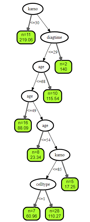
###设置树的个数为3:
## plot tree number 3
plot(get.tree(v.obj, 3))
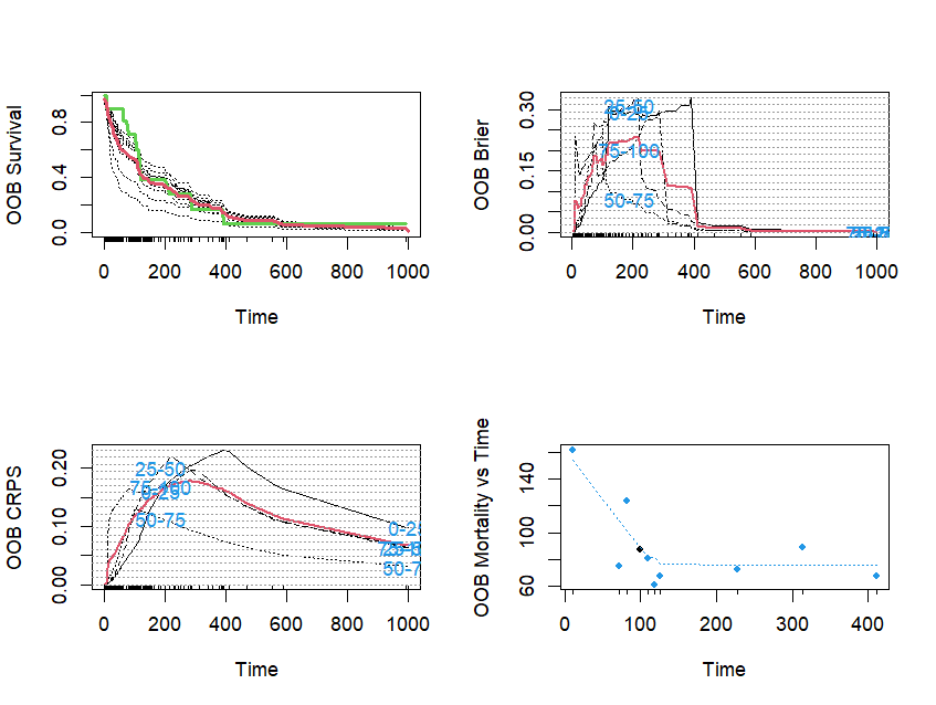
###绘制训练森林的结果
## plot results of trained forest
plot(v.obj)
##
## Importance Relative Imp
## karno 0.2093 1.0000
## celltype 0.0689 0.3292
## age 0.0291 0.1389
## diagtime 0.0248 0.1187
## trt 0.0028 0.0134
## prior -0.0008 -0.0037

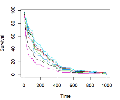
直接绘制前10个个体的生存曲线
## plot survival curves for first 10 individuals -- direct way
matplot(v.obj$time.interest, 100 * t(v.obj$survival.oob[1:10, ]), xlab = "Time",
    ylab = "Survival", type = "l", lty = 1)
##使用函数plot.survival绘制前10个个体的生存曲线
## plot survival curves for first 10 individuals using function 'plot.survival'
plot.survival(v.obj, subset = 1:10)
## fast nodesize optimization for veteran data optimal nodesize in survival is
## larger than other families see the function 'tune' for more examples
tune.nodesize(Surv(time, status) ~ ., veteran)
## nodesize =  1  OOB error = 32.03%
## nodesize =  2  OOB error = 31.5%
## nodesize =  3  OOB error = 31.43%
## nodesize =  4  OOB error = 31.09%
## nodesize =  5  OOB error = 29.94%
## nodesize =  6  OOB error = 30.18%
## nodesize =  7  OOB error = 30.23%
## nodesize =  8  OOB error = 30.52%
## nodesize =  9  OOB error = 32.17%
## nodesize =  10  OOB error = 31.44%
## nodesize =  15  OOB error = 30.41%
## nodesize =  20  OOB error = 30.2%
## nodesize =  25  OOB error = 29.29%
## nodesize =  30  OOB error = 30.07%
## nodesize =  35  OOB error = 32.59%
## nodesize =  40  OOB error = 31.23%
## optimal nodesize: 25
## $nsize.opt
## [1] 25
##
## $err
##    nodesize       err
## 1         1 0.3203098
## 2         2 0.3149949
## 3         3 0.3143164
## 4         4 0.3109239
## 5         5 0.2993893
## 6         6 0.3017641
## 7         7 0.3023295
## 8         8 0.3051566
## 9         9 0.3216669
## 10       10 0.3144295
## 11       15 0.3041389
## 12       20 0.3019903
## 13       25 0.2929436
## 14       30 0.3007464
## 15       35 0.3258510
## 16       40 0.3122809
###快速优化老数据的节点大小##最优的生存节点大小比其他家族##查看函数“tune”了解更多示例
## fast nodesize optimization for veteran data optimal nodesize in survival is
## larger than other families see the function 'tune' for more examples
tune.nodesize(Surv(time, status) ~ ., veteran)
## nodesize =  1  OOB error = 32.16%
## nodesize =  2  OOB error = 30.61%
## nodesize =  3  OOB error = 30.69%
## nodesize =  4  OOB error = 29.75%
## nodesize =  5  OOB error = 30.27%
## nodesize =  6  OOB error = 30.87%
## nodesize =  7  OOB error = 28.97%
## nodesize =  8  OOB error = 28.85%
## nodesize =  9  OOB error = 29.69%
## nodesize =  10  OOB error = 30.06%
## nodesize =  15  OOB error = 30.73%
## nodesize =  20  OOB error = 31.4%
## nodesize =  25  OOB error = 31.4%
## nodesize =  30  OOB error = 30.73%
## nodesize =  35  OOB error = 32.71%
## nodesize =  40  OOB error = 31.85%
## optimal nodesize: 8
## $nsize.opt
## [1] 8
##
## $err
##    nodesize       err
## 1         1 0.3215538
## 2         2 0.3060613
## 3         3 0.3068529
## 4         4 0.2974669
## 5         5 0.3026688
## 6         6 0.3086622
## 7         7 0.2896641
## 8         8 0.2885333
## 9         9 0.2969015
## 10       10 0.3006333
## 11       15 0.3073052
## 12       20 0.3139772
## 13       25 0.3139772
## 14       30 0.3073052
## 15       35 0.3270949
## 16       40 0.3185005
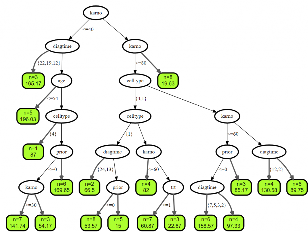
2.2 例子二
vd <- veteran
vd$celltype = factor(vd$celltype)
vd$diagtime = factor(vd$diagtime)
vd.obj <- rfsrc(Surv(time, status) ~ ., vd, ntree = 100, nodesize = 5)
plot(get.tree(vd.obj, 3))
2. 原发性胆汁性肝硬化(PBC)
2.1. 例子一
## Primary biliary cirrhosis (PBC) of the liver
pbc.obj <- rfsrc(Surv(days, status) ~ ., pbc)
print(pbc.obj)
##                          Sample size: 276
##                     Number of deaths: 111
##                      Number of trees: 500
##            Forest terminal node size: 15
##        Average no. of terminal nodes: 14.038
## No. of variables tried at each split: 5
##               Total no. of variables: 17
##        Resampling used to grow trees: swor
##     Resample size used to grow trees: 174
##                             Analysis: RSF
##                               Family: surv
##                       Splitting rule: logrank *random*
##        Number of random split points: 10
##                           (OOB) CRPS: 0.1259854
##    (OOB) Requested performance error: 0.16910578
2.2. 例子二
pbc.obj2 <- rfsrc(Surv(days, status) ~ ., pbc, nsplit = 10, na.action = "na.impute")

## same as above but iterate the missing data algorithm
pbc.obj3 <- rfsrc(Surv(days, status) ~ ., pbc, na.action = "na.impute", nimpute = 3)

## fast way to impute data (no inference is done) see impute for more details
pbc.imp <- impute(Surv(days, status) ~ ., pbc, splitrule = "random")
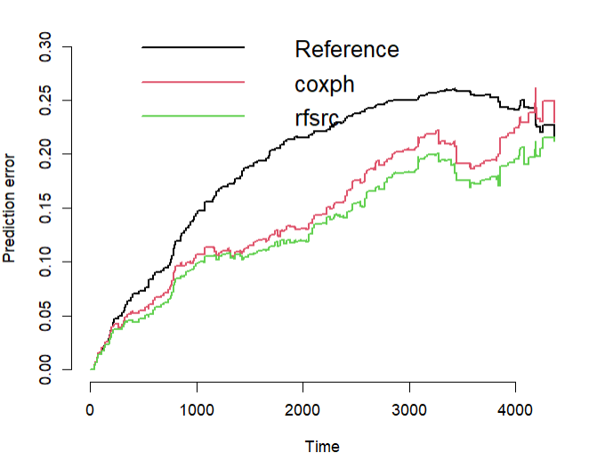
3. 比较RF-SRC和Cox回归
比较RF-SRC和Cox回归,说明性能的c指数和Brier评分措施,假设加载了“pec”和“survival”
require("survival")
require("pec")
require("prodlim")

## prediction function required for pec
predictSurvProb.rfsrc <- function(object, newdata, times, ...) {
    ptemp <- predict(object, newdata = newdata, ...)$survival
    pos <- sindex(jump.times = object$time.interest, eval.times = times)
    p <- cbind(1, ptemp)[, pos + 1]
    if (NROW(p) != NROW(newdata) || NCOL(p) != length(times))
        stop("Prediction failed")
    p
}

## data, formula specifications
data(pbc, package = "randomForestSRC")
pbc.na <- na.omit(pbc)  ##remove NA's
surv.f <- as.formula(Surv(days, status) ~ .)
pec.f <- as.formula(Hist(days, status) ~ 1)

## run cox/rfsrc models for illustration we use a small number of trees
cox.obj <- coxph(surv.f, data = pbc.na, x = TRUE)
rfsrc.obj <- rfsrc(surv.f, pbc.na, ntree = 150)

## compute bootstrap cross-validation estimate of expected Brier score see
## Mogensen, Ishwaran and Gerds (2012) Journal of Statistical Software
set.seed(17743)
prederror.pbc <- pec(list(cox.obj, rfsrc.obj), data = pbc.na, formula = pec.f, splitMethod = "bootcv",
    B = 50)
print(prederror.pbc)
##
## Prediction error curves
##
## Prediction models:
##
## Reference     coxph     rfsrc
## Reference     coxph     rfsrc
##
## Right-censored response of a survival model
##
## No.Observations: 276
##
## Pattern:
##                 Freq
##  event          111
##  right.censored 165
##
## IPCW: marginal model
##
## Method for estimating the prediction error:
##
## Bootstrap cross-validation
##
## Type: resampling
## Bootstrap sample size:  276
## No. bootstrap samples:  50
## Sample size:  276
##
## Cumulative prediction error, aka Integrated Brier score  (IBS)
##  aka Cumulative rank probability score
##
## Range of integration: 0 and time=4365 :
##
##
## Integrated Brier score (crps):
##
##           IBS[0;time=4365)
## Reference            0.191
## coxph                0.146
## rfsrc                0.132
plot(prederror.pbc)
## compute out-of-bag C-index for cox regression and compare to rfsrc
rfsrc.obj <- rfsrc(surv.f, pbc.na)
cat("out-of-bag Cox Analysis ...", "\n")
## out-of-bag Cox Analysis ...
cox.err <- sapply(1:100, function(b) {
    if (b%%10 == 0)
        cat("cox bootstrap:", b, "\n")
    train <- sample(1:nrow(pbc.na), nrow(pbc.na), replace = TRUE)
    cox.obj <- tryCatch({
        coxph(surv.f, pbc.na[train, ])
    }, error = function(ex) {
        NULL
    })
    if (!is.null(cox.obj)) {
        get.cindex(pbc.na$days[-train], pbc.na$status[-train], predict(cox.obj, pbc.na[-train,
            ]))
    } elseNA
})
## cox bootstrap: 10
## cox bootstrap: 20
## cox bootstrap: 30
## cox bootstrap: 40
## cox bootstrap: 50
## cox bootstrap: 60
## cox bootstrap: 70
## cox bootstrap: 80
## cox bootstrap: 90
## cox bootstrap: 100
cat("\n\tOOB error rates\n\n")
##
## 	OOB error rates
cat("\tRSF            : ", rfsrc.obj$err.rate[rfsrc.obj$ntree], "\n")
## 	RSF            :  0.1714494
cat("\tCox regression : ", mean(cox.err, na.rm = TRUE), "\n")
## 	Cox regression :  0.1938652
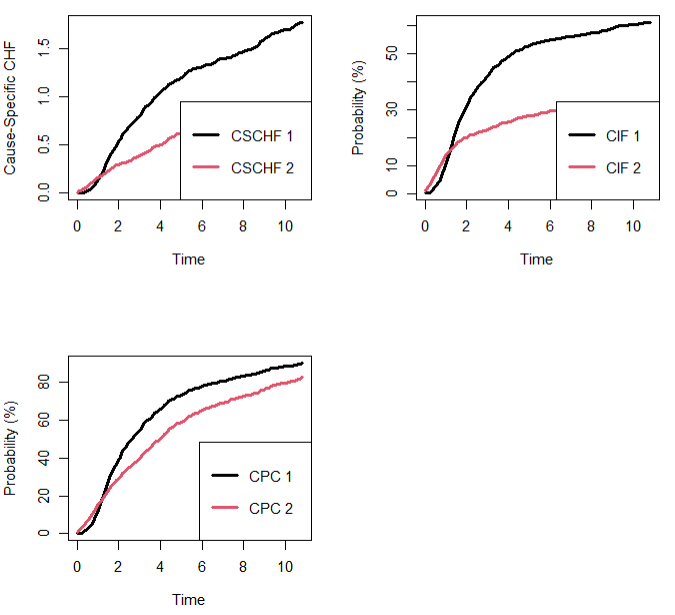
4. 妇女跨机构艾滋病毒研究
生存竞争风险比例模型
wihs.obj <- rfsrc(Surv(time, status) ~ ., wihs, nsplit = 3, ntree = 100)
plot.competing.risk(wihs.obj)
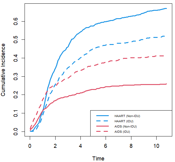
cif <- wihs.obj$cif.oob
Time <- wihs.obj$time.interest
idu <- wihs$idu
cif.haart <- cbind(apply(cif[, , 1][idu == 0, ], 2, mean), apply(cif[, , 1][idu ==
    1, ], 2, mean))
cif.aids <- cbind(apply(cif[, , 2][idu == 0, ], 2, mean), apply(cif[, , 2][idu ==
    1, ], 2, mean))
matplot(Time, cbind(cif.haart, cif.aids), type = "l", lty = c(1, 2, 1, 2), col = c(4,
    4, 2, 2), lwd = 3, ylab = "Cumulative Incidence")
legend("bottomright", legend = c("HAART (Non-IDU)", "HAART (IDU)", "AIDS (Non-IDU)",
    "AIDS (IDU)"), lty = c(1, 2, 1, 2), col = c(4, 4, 2, 2), lwd = 3, cex = 0.6)
结果解读
随机生存森林可以对变量重要性进行排名,VIMP法和最小深度法是最常用的方法:变量VIMP值小于0说明该变量降低了预测的准确性,而当VIMP值大于0则说明该变量提高了预测的准确性;最小深度法通过计算运行到最终节点时的最小深度来给出各变量对于结局事件的重要性。
下图为综合两种方法的散点图,其中,蓝色点代表VIMP值大于0,红色则代表VIMP值小于0;在红色对角虚线上的点代表两种方法对该变量的排名相同,高于对角虚线的点代表其VIMP排名更高,低于对角虚线的点则代表其最小深度排名更高。相较于Cox比例风险回归模型等传统生存分析方法,随机生存森林模型的预测准确度至少等同或优于传统生存分析方法。随机生存森林模型的优势体现在它不受比例风险假定、对数线性假定等条件的约束。同时,随机生存森林具备一般随机森林的优点,能够通过两个随机采样的过程来防止其算法的过度拟合问题。除此之外,随机生存森林还能够对高维数据进行生存分析和变量筛选,也能够应用于对竞争风险(competing risk)的分析。因而,随机生存森林模型有着更为广泛的研究空间。
但是随机生存森林也存在缺陷:易受离群值的影响。分析中有离群值数据时,预测准确度会稍劣于传统生存分析方法。Cox比例风险回归模型对于生存数据的分析不仅仅用于预测,还可以较为便捷地给出各变量与生存结局的关系,所以随机生存森林模型应该和传统生存分析相结合应用,并不能完全替代传统生存分析模型。
更多关于这个软件的用法可以参考如下资源: