1 Quick Start with Guitar
if (!requireNamespace("BiocManager", quietly = TRUE))
    install.packages("BiocManager")

BiocManager::install("Guitar")
This is a manual for Guitar package. The Guitar package is aimed for RNA landmark-guided transcriptomic analysis of RNA-reated genomic features. The Guitar package enables the comparison of multiple genomic features, which need to be stored in a name list. Please see the following example, which reads 1000 RNA m6A methylation sites into R for detection. Of course, in actual data analysis, features may come from multiple sets of resources.
library(Guitar)

# genomic features imported into named list

stBedFiles <- list(system.file("extdata", "m6A_mm10_exomePeak_1000peaks_bed12.bed",

package="Guitar"))
With the following script, we may generate the transcriptomic distribution of genomic features to be tested, and the result will be automatically saved into a PDF file under the working directory with prefix “example”. With the GuitarPlot function, the gene annotation can be downloaded from internet automatically with a genome assembly number provided; however, this feature requires working internet and might take a longer time. The toy Guitar coordinates generated internally should never be re-used in other real data analysis.
count <- GuitarPlot(txGenomeVer = "mm10",

stBedFiles = stBedFiles,

miscOutFilePrefix = NA)
In a more efficent protocol, in order to re-use the gene annotation and Guitar coordinates, you will have to build Guitar Coordiantes from a txdb object in a separate step. The transcriptDb contains the gene annotation information and can be obtained in a number of ways, .e.g, download the complete gene annotation of species from UCSC automatically, which might takes a few minutes. In the following analysis, we load the Txdb object from a toy dataset provided with the Guitar package. Please note that this is only a very small part of the complete hg19 transcriptome, and the Txdb object provided with Guitar package should not be used in real data analysis. With a TxDb object that contains gene annotation information, we in the next build Guitar coordiantes, which is essentially a bridge connects the transcriptomic landmarks and genomic coordinates.
txdb_file <- system.file("extdata", "mm10_toy.sqlite",
package="Guitar")
txdb <- loadDb(txdb_file)
guitarTxdb <- makeGuitarTxdb(txdb = txdb, txPrimaryOnly = FALSE)
You may now generate the Guitar plot from the named list of genome-based features.
GuitarPlot(txTxdb = txdb,
stBedFiles = stBedFiles,
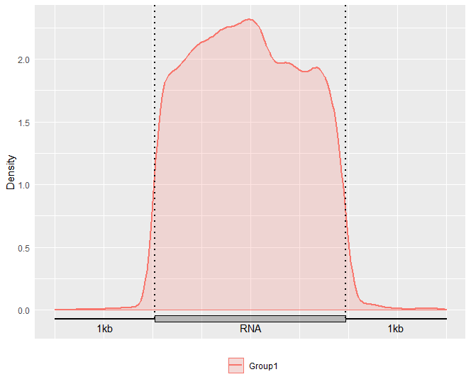
miscOutFilePrefix = "example")Alternatively, you may also optionally include the promoter DNA region and tail DNA region on the 5’ and 3’ side of a transcript in the plot with parameter headOrtail =TRUE.
GuitarPlot(txTxdb = txdb,

stBedFiles = stBedFiles,

headOrtail = TRUE)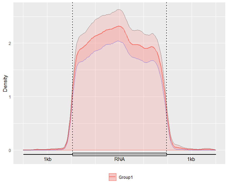
Alternatively, you may also optionally include the Confidence Interval for guitar plot with parameter enableCI = FALSE.
GuitarPlot(txTxdb = txdb,

stBedFiles = stBedFiles,

headOrtail = TRUE,

enableCI = FALSE)
2 Supported Data Format
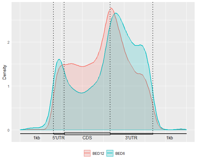
Besides BED file, Guitar package also supports GRangesList and GRanges data structures. Please see the following examples.
# import different data formats into a named list object.

# These genomic features are using mm10 genome assembly

stBedFiles <- list(system.file("extdata", "m6A_mm10_exomePeak_1000peaks_bed12.bed",

package="Guitar"),

system.file("extdata", "m6A_mm10_exomePeak_1000peaks_bed6.bed",

package="Guitar"))

# Build Guitar Coordinates

txdb_file <- system.file("extdata", "mm10_toy.sqlite",

package="Guitar")

txdb <- loadDb(txdb_file)

# Guitar Plot

GuitarPlot(txTxdb = txdb,

stBedFiles = stBedFiles,

headOrtail = TRUE,

enableCI = FALSE,

mapFilterTranscript = TRUE,

pltTxType = c("mrna"),

stGroupName = c("BED12","BED6"))
3 Processing of sampling sites information
We can select parameters for site sampling.
stGRangeLists = vector("list", length(stBedFiles))

sitesPoints <- list()

for (i in seq_len(length(stBedFiles))) {

stGRangeLists[[i]] <- blocks(import(stBedFiles[[i]]))

}

for (i in seq_len(length(stGRangeLists))) {

sitesPoints[[i]] <- samplePoints(stGRangeLists[i],

stSampleNum = 10,

stAmblguity = 5,

pltTxType = c("mrna"),

stSampleModle = "Equidistance",

mapFilterTranscript = FALSE,

guitarTxdb = guitarTxdb)

}
4 Guitar Coordinates – Transcriptomic Landmarks Projected on Genome
The guitarTxdb object contains the genome-projected transcriptome coordinates, which can be valuable for evaluating transcriptomic information related applications, such as checking the quality of MeRIP-Seq data. The Guitar coordinates are essentially the genomic projection of standardized transcript-based coordiantes, making a viable bridge beween the landmarks on transcript and genome-based coordinates. It is based on the txdb object input, extracts the transcript information in txdb, selects the transcripts that match the parameters according to the component parameters set by the user, and saves according to the transcript type (tx, mrna, ncrna).
guitarTxdb <- makeGuitarTxdb(txdb = txdb,

txAmblguity = 5,

txMrnaComponentProp = c(0.1,0.15,0.6,0.05,0.1),

txLncrnaComponentProp = c(0.2,0.6,0.2),

pltTxType = c("tx","mrna","ncrna"),

txPrimaryOnly = FALSE)
5 Check the Overlapping between Different Components
We can also check the distribution of the Guitar coordinates built.
gcl <- list(guitarTxdb$tx$tx)

GuitarPlot(txTxdb = txdb,

stGRangeLists = gcl,

stSampleNum = 200,

enableCI = TRUE,

pltTxType = c("tx"),

txPrimaryOnly = FALSE

)

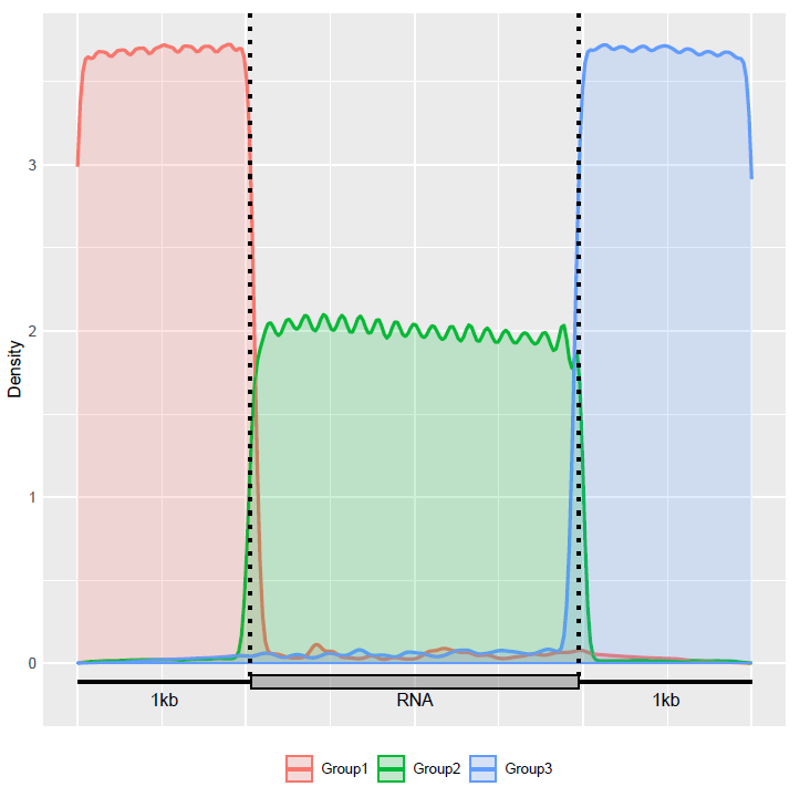
Alternatively, we can extract the RNA components, check the distribution of tx components in the transcriptome.
GuitarCoords <- guitarTxdb$tx$txComponentGRange

type <- paste(mcols(GuitarCoords)$componentType,mcols(GuitarCoords)$txType)

key <- unique(type)

landmark <- list(1,2,3,4,5,6,7,8,9,10,11)

names(landmark) <- key

for (i in 1:length(key)) {

landmark[[i]] <- GuitarCoords[type==key[i]]

}

GuitarPlot(txTxdb = txdb ,

stGRangeLists = landmark[1:3],

pltTxType = c("tx"),

enableCI = FALSE

)
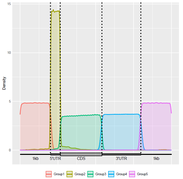
Check the distribution of mRNA components in the transcriptome
GuitarPlot(txTxdb = txdb ,

stGRangeLists = landmark[4:8],

pltTxType = c("mrna"),

enableCI = FALSE

)
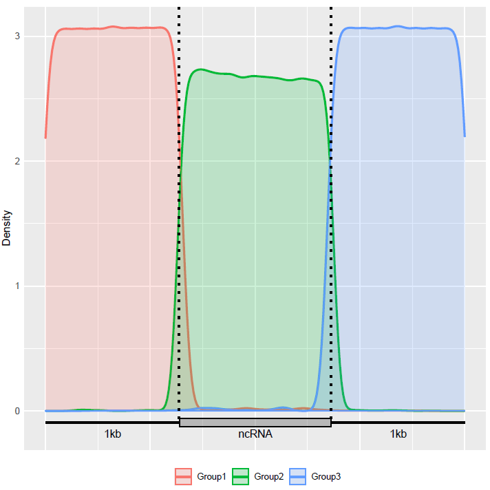
Check the distribution of lncRNA components in the transcriptome
GuitarPlot(txTxdb = txdb ,

stGRangeLists = landmark[9:11],

pltTxType = c("ncrna"),

enableCI = FALSE

)
6 Session Information
sessionInfo()
进哥,我遇到个问题,麻烦你帮我看一下,我找了好久还是没发现是哪里的问题:
这是我的代码:
library(Guitar)
package.version(“Guitar”)
library(dplyr, verbose = F)
#BiocManager::install(“Guitar”)
setwd(“/Users/liyangjun/Desktop/m6A-seq/Results-2”)
#makeTxDbFromGFF:这个函数来自GenomicFeatures包,用于从GTF文件创建转录数据库(txdb),
#这个数据库包含了基因、转录本、外显子等的注释信息。这是为了后续的基因组注释和数据映射。
txdb <- makeTxDbFromGFF("gencode.v44.annotation.gtf")
#stBedFiles:从snakemake工作流获取的输入文件路径,
#这里假设是BED格式的文件,包含了m6A修饰位点的数据。
stBedFiles <- "SRR_totalm6A.FDR.filtered_0.005_10mer.bed"
#miscOutFilePrefix:设置输出文件前缀,用于GuitarPlot函数输出结果的命名
miscOutFilePrefix <- paste0("GuitarPlot_", stBedFiles)
#GuitarPlot函数是Guitar包的核心功能,用于生成可视化图。这个函数的参数设置了如何创建图表:
#txTxdb:提供了转录数据库。
# stBedFiles:提供了BED格式的输入文件。
# headOrtail:设置为TRUE,表示可能只关注转录本的头部或尾部。
# enableCI:设置为FALSE,表示不绘制置信区间。
# mapFilterTranscript:设置为TRUE,表示在映射到转录本时进行过滤。
# stGroupName:为可视化图中的数据组设置名称。
# pltTxType:设置为c("mrna"),表示只绘制mRNA类型的转录本。
# miscOutFilePrefix:设置输出文件的前缀,这将影响输出文件的命名。
GuitarPlot(txTxdb = txdb,
stBedFiles = stBedFiles,
headOrtail = TRUE,
enableCI = FALSE,
mapFilterTranscript = TRUE,
stGroupName = stBedFiles,
pltTxType = c("mrna"),
miscOutFilePrefix = miscOutFilePrefix)
平台:mac x86
数据:bed文件比较特殊,我的区段只有2bp,因为我得到的其实是位点信息,然后来将位点-1作为start,我是想看我得到的单碱基位点的m6A修饰位点的分布图。
报错:
Error in density.default(siteID, adjust = adjust, from = 0, to = 1, n = 256, :
'x' contains missing values
In addition: There were 50 or more warnings (use warnings() to see the first 50)
我也遇到了同样的问题,我的bed位点是单碱基的信息,请问您解决了吗?
博主您好,我想请问一下,这个包可用于绘制每个样本的reads在不同exon上的分布趋势吗?
您好,意思是CDS区不同外显子上的分布?这个我没有试过,理论上只要有对应的坐标都可以的,我有空试试
您好!请问您有没有碰到过这个问题:Error in h(simpleError(msg, call)) :
在为’blocks’函数选择方法时评估’x’参数出了错: color intensity NA, not in 0:255,,,要如何解决?谢谢!
请问具体是哪一步报错,贴上来一起学习研究呗