1引言
今天分享一个绘制转录本的 R 包 ggtranscript。
githup 地址:
https://github.com/dzhang32/ggtranscript参考手册:
https://dzhang32.github.io/ggtranscript/articles/ggtranscript.html
 包含
包含 geom_range(), geom_half_range(), geom_intron(), geom_junction() 和 geom_junction_label_repel() 五个函数。
2安装
# you can install the development version of ggtranscript from GitHub:
# install.packages("devtools")
devtools::install_github("dzhang32/ggtranscript")3输入数据类型
library(magrittr)
library(ggtranscript)
library(ggplot2)4输入数据类型:
可以参考 GTF 格式文件:
sod1_annotation %>% head()
#> # A tibble: 6 × 8
#>   seqnames  start    end strand type  gene_name transcript_name transcript_biot…
#>
#> 1 21       3.17e7 3.17e7 +      gene  SOD1      NA              NA
#> 2 21       3.17e7 3.17e7 +      tran… SOD1      SOD1-202        protein_coding
#> 3 21       3.17e7 3.17e7 +      exon  SOD1      SOD1-202        protein_coding
#> 4 21       3.17e7 3.17e7 +      CDS   SOD1      SOD1-202        protein_coding
#> 5 21       3.17e7 3.17e7 +      star… SOD1      SOD1-202        protein_coding
#> 6 21       3.17e7 3.17e7 +      exon  SOD1      SOD1-202        protein_coding

pknox1_annotation %>% head()
#> # A tibble: 6 × 8
#>   seqnames  start    end strand type  gene_name transcript_name transcript_biot…
#>
#> 1 21       4.30e7 4.30e7 +      gene  PKNOX1    NA              NA
#> 2 21       4.30e7 4.30e7 +      tran… PKNOX1    PKNOX1-203      protein_coding
#> 3 21       4.30e7 4.30e7 +      exon  PKNOX1    PKNOX1-203      protein_coding
#> 4 21       4.30e7 4.30e7 +      exon  PKNOX1    PKNOX1-203      protein_coding
#> 5 21       4.30e7 4.30e7 +      exon  PKNOX1    PKNOX1-203      protein_coding
#> 6 21       4.30e7 4.30e7 +      exon  PKNOX1    PKNOX1-203      protein_coding

sod1_junctions
#> # A tibble: 5 × 5
#>   seqnames    start      end strand mean_count
#>
#> 1 chr21    31659787 31666448 +           0.463
#> 2 chr21    31659842 31660554 +           0.831
#> 3 chr21    31659842 31663794 +           0.316
#> 4 chr21    31659842 31667257 +           4.35
#> 5 chr21 31660351 31663789 + 0.3245绘制外显子和内含子
# 内置数据
sod1_annotation %>% head()
#> # A tibble: 6 × 8
#> seqnames start end strand type gene_name transcript_name transcript_biot…
#>
#> 1 21 3.17e7 3.17e7 + gene SOD1 NA NA
#> 2 21 3.17e7 3.17e7 + tran… SOD1 SOD1-202 protein_coding
#> 3 21 3.17e7 3.17e7 + exon SOD1 SOD1-202 protein_coding
#> 4 21 3.17e7 3.17e7 + CDS SOD1 SOD1-202 protein_coding
#> 5 21 3.17e7 3.17e7 + star… SOD1 SOD1-202 protein_coding
#> 6 21 3.17e7 3.17e7 + exon SOD1 SOD1-202 protein_coding
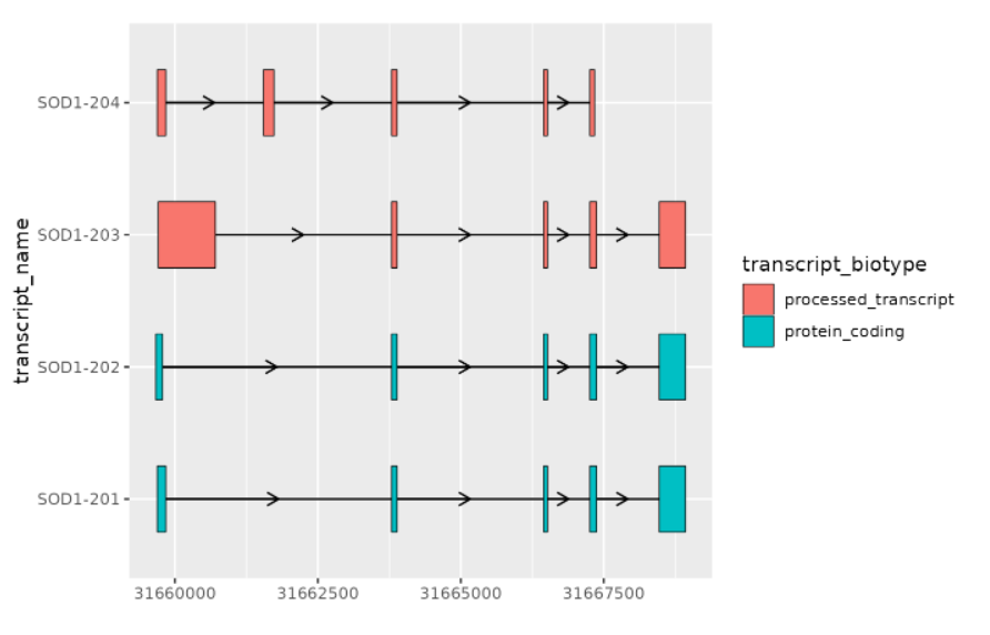
# extract exons
# 筛选外显子
sod1_exons % dplyr::filter(type == "exon")
# 绘图
sod1_exons %>%
ggplot(aes(
xstart = start,
xend = end,
y = transcript_name
)) +
geom_range(
aes(fill = transcript_biotype)
) +
geom_intron(
data = to_intron(sod1_exons, "transcript_name"),
aes(strand = strand)
)
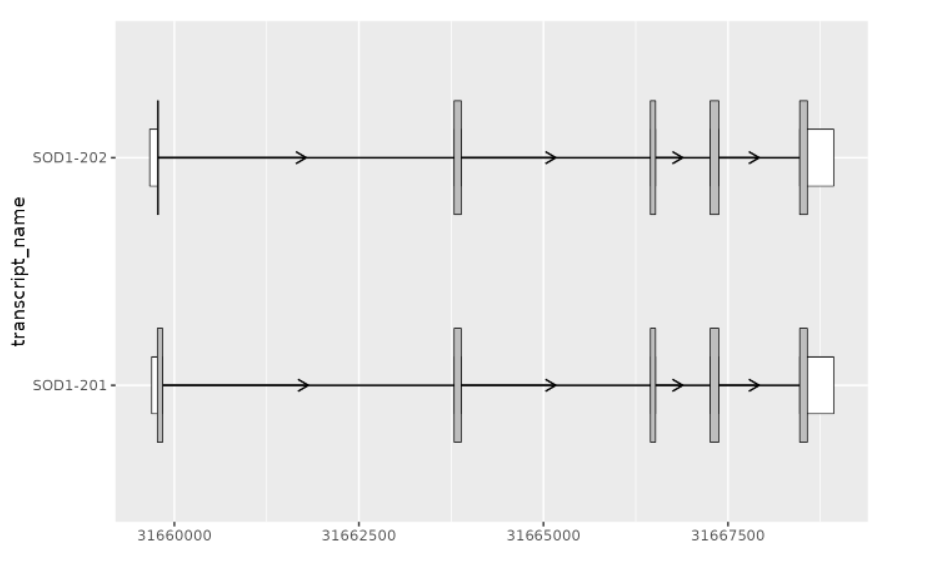
6绘制 UTR 和 CDS 结构
# filter for only exons from protein coding transcripts
sod1_exons_prot_cod %
    dplyr::filter(transcript_biotype == "protein_coding")

# obtain cds
sod1_cds % dplyr::filter(type == "CDS")

sod1_exons_prot_cod %>%
    ggplot(aes(
        xstart = start,
        xend = end,
        y = transcript_name
    )) +
    geom_range(
        fill = "white",
        height = 0.25
    ) +
    geom_range(
        data = sod1_cds
    ) +
    geom_intron(
        data = to_intron(sod1_exons_prot_cod, "transcript_name"),
        aes(strand = strand),
        arrow.min.intron.length = 500,
    )
7绘制 junctions
# extract exons and cds for the MANE-select transcript
sod1_201_exons % dplyr::filter(transcript_name == "SOD1-201")
sod1_201_cds % dplyr::filter(transcript_name == "SOD1-201")

# add transcript name column to junctions for plotting
sod1_junctions % dplyr::mutate(transcript_name = "SOD1-201")

sod1_201_exons %>%
  ggplot(aes(
    xstart = start,
    xend = end,
    y = transcript_name
  )) +
  geom_range(
    fill = "white",
    height = 0.25
  ) +
  geom_range(
    data = sod1_201_cds
  ) +
  geom_intron(
    data = to_intron(sod1_201_exons, "transcript_name")
  ) +
  geom_junction(
    data = sod1_junctions,
    aes(size = mean_count),
    junction.y.max = 0.5
  ) +
  geom_junction_label_repel(
    data = sod1_junctions,
    aes(label = round(mean_count, 2)),
    junction.y.max = 0.5
  ) +
  scale_size_continuous(range = c(0.1, 1))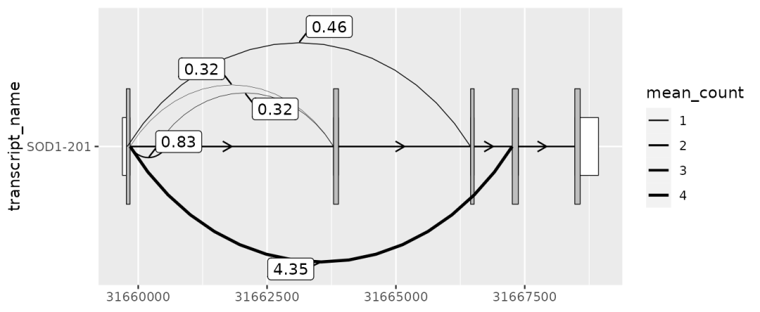
8可视化转录本结构差异
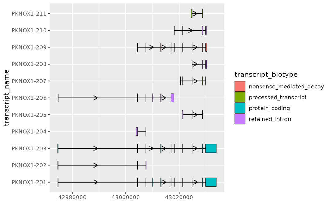
有些基因的内含子很长,可以使用 arrow.min.intron.length 参数控制最小内含子长度来更好的可视化:
# extract exons
pknox1_exons % dplyr::filter(type == "exon")

pknox1_exons %>%
    ggplot(aes(
        xstart = start,
        xend = end,
        y = transcript_name
    )) +
    geom_range(
        aes(fill = transcript_biotype)
    ) +
    geom_intron(
        data = to_intron(pknox1_exons, "transcript_name"),
        aes(strand = strand),
        arrow.min.intron.length = 3500
    )
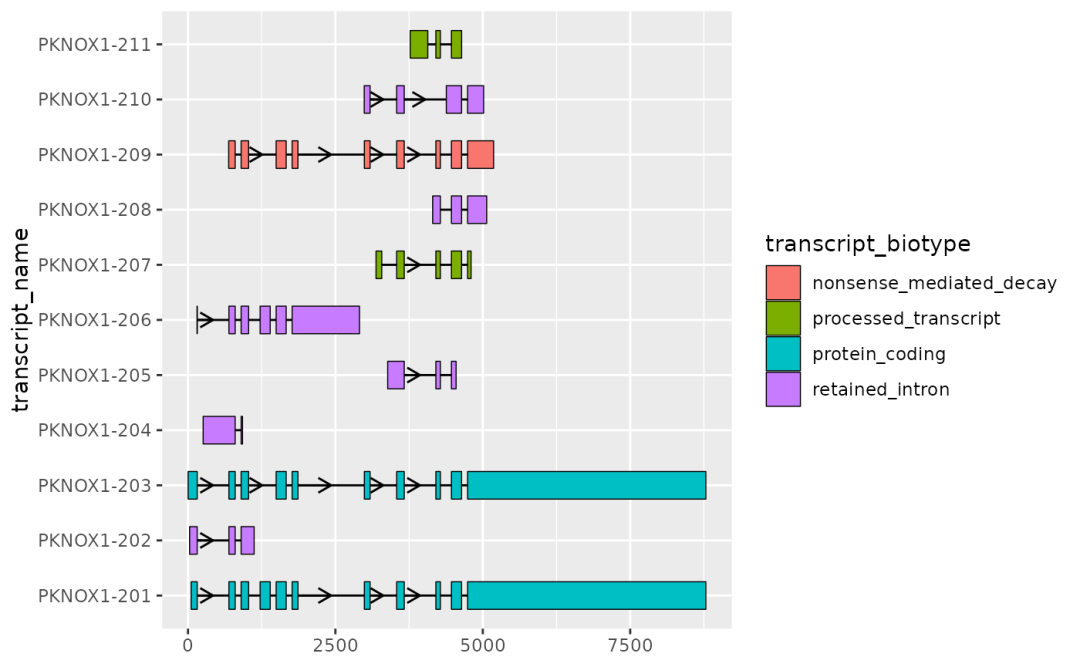
9优化可视化效果
使用 shorten_gaps 函数来减少外显子之间的间距,更好的展示外显子结构:
# extract exons
pknox1_exons % dplyr::filter(type == "exon")

pknox1_rescaled   exons = pknox1_exons,
  introns = to_intron(pknox1_exons, "transcript_name"),
  group_var = "transcript_name"
)

# shorten_gaps() returns exons and introns all in one data.frame()
# let's split these for plotting
pknox1_rescaled_exons % dplyr::filter(type == "exon")
pknox1_rescaled_introns % dplyr::filter(type == "intron")

pknox1_rescaled_exons %>%
    ggplot(aes(
        xstart = start,
        xend = end,
        y = transcript_name
    )) +
    geom_range(
        aes(fill = transcript_biotype)
    ) +
    geom_intron(
        data = pknox1_rescaled_introns,
        aes(strand = strand),
        arrow.min.intron.length = 300
    )
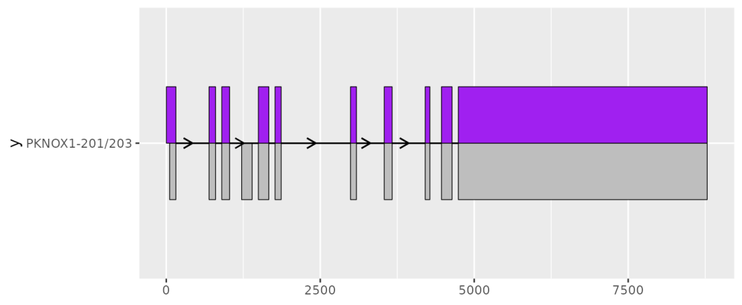
10比较两个转录本
geom_half_range 可以比较两个转录本结构:
# extract the two transcripts to be compared
pknox1_rescaled_201_exons %
  dplyr::filter(transcript_name == "PKNOX1-201")
pknox1_rescaled_203_exons %
  dplyr::filter(transcript_name == "PKNOX1-203")

pknox1_rescaled_201_exons %>%
    ggplot(aes(
        xstart = start,
        xend = end,
        y = "PKNOX1-201/203"
    )) +
    geom_half_range() +
    geom_intron(
        data = to_intron(pknox1_rescaled_201_exons, "transcript_name"),
        arrow.min.intron.length = 300
    ) +
    geom_half_range(
        data = pknox1_rescaled_203_exons,
        range.orientation = "top",
        fill = "purple"
    ) +
    geom_intron(
        data = to_intron(pknox1_rescaled_203_exons, "transcript_name"),
        arrow.min.intron.length = 300
    )
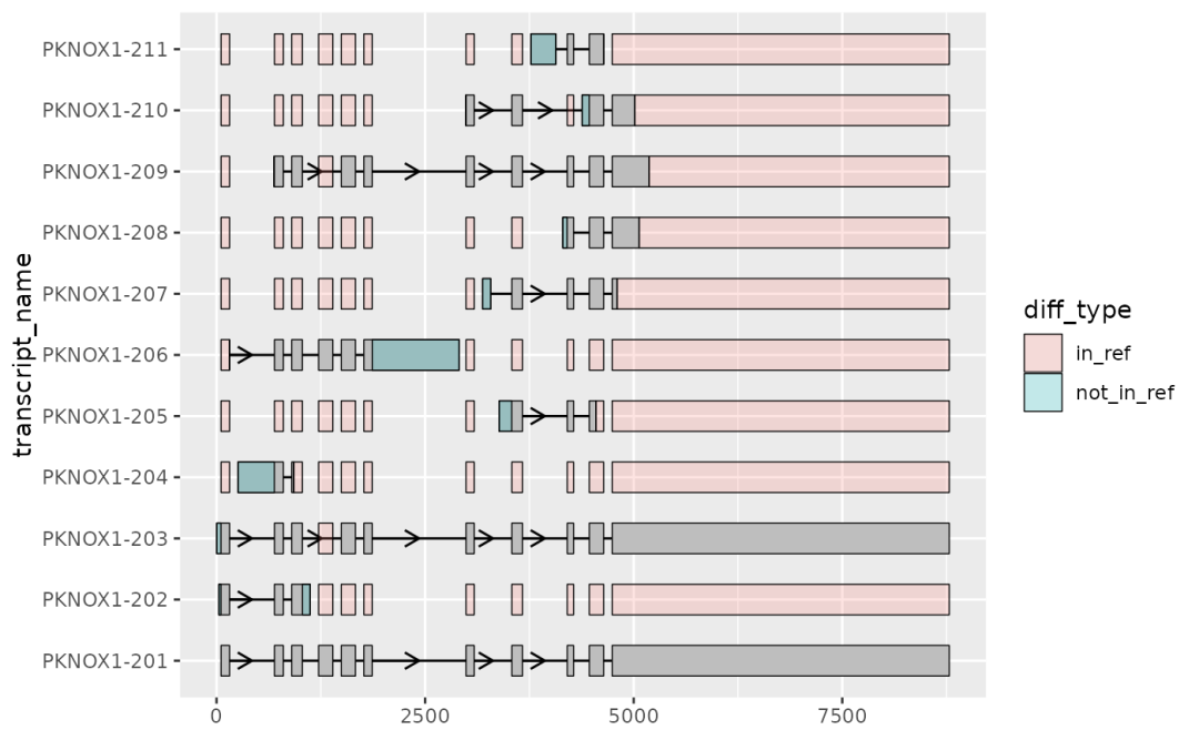
11多个转录本与参考转录本比较
to_diff 函数可以使多个转录本与指定参考转录本结构比较:
mane
not_mane %
  dplyr::filter(transcript_name != "PKNOX1-201")

pknox1_rescaled_diffs     exons = not_mane,
    ref_exons = mane,
    group_var = "transcript_name"
)

pknox1_rescaled_exons %>%
    ggplot(aes(
        xstart = start,
        xend = end,
        y = transcript_name
    )) +
    geom_range() +
    geom_intron(
        data = pknox1_rescaled_introns,
        arrow.min.intron.length = 300
    ) +
    geom_range(
        data = pknox1_rescaled_diffs,
        aes(fill = diff_type),
        alpha = 0.2
    )
进哥,ggtranscript这个包没办法安装啊