本文转载自:R语言GEO数据挖掘02-解决GEO数据中的多个探针对应一个基因 – 简书
- 当我们来到这一步时我们默认经过前期的处理,你已经获得了表达矩阵的数据,获得了探针的注释信息。
- 在进一步探索过程中我们发现了一个存在多个探针对应一个基因的情况,这是本文需要解决的问题
- 解决的办法可以是取多个探针中的最大值,也可以是平均值,中位值等等,都存在一定的道理。这同时也提示了我们高通量数据的筛选性质,存在很大的不确定性,并不是基因定量的金标准,常常发生芯片或者测序的结果有些难以得到验证的情况。
- 本文将通过四种方式来完成取多个探针的平均值作为表达的目的,当然如果想用最大值,直接将 mean换成 max即可。
载入数据
library(dplyr)
##
## Attaching package: 'dplyr'
## The following objects are masked from 'package:stats':
##
##     filter, lag
## The following objects are masked from 'package:base':
##
##     intersect, setdiff, setequal, union
##

if(T){
load("expma.Rdata")
load("probe.Rdata")
}
expma[1:5,1:5]
##           GSM188013 GSM188014 GSM188016 GSM188018 GSM188020
## 1007_s_at 15630.200 17048.800 13667.500 15138.800 10766.600
## 1053_at    3614.400  3563.220  2604.650  1945.710  3371.290
## 117_at     1032.670  1164.150   510.692  5061.200   452.166
## 121_at     5917.800  6826.670  4562.440  5870.130  3869.480
## 1255_g_at   224.525   395.025   207.087   164.835   111.609
boxplot(expma)##看下表达情况
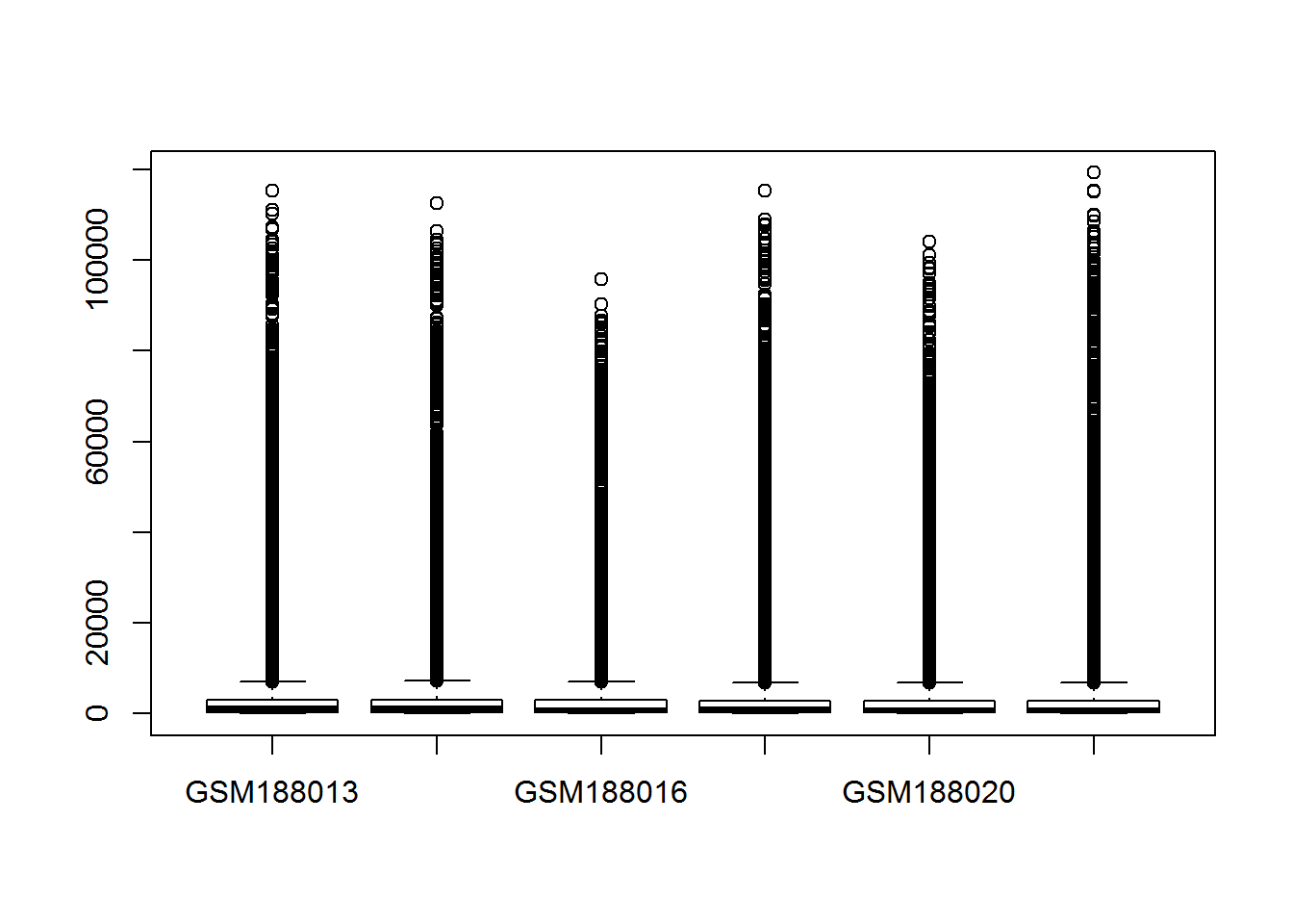
Fig1
metadata信息
metdata[1:5,1:5]
##                                                              title
## GSM188013   DMSO treated MCF7 breast cancer cells [HG-U133A] Exp 1
## GSM188014 Dioxin treated MCF7 breast cancer cells [HG-U133A] Exp 1
## GSM188016   DMSO treated MCF7 breast cancer cells [HG-U133A] Exp 2
## GSM188018 Dioxin treated MCF7 breast cancer cells [HG-U133A] Exp 2
## GSM188020   DMSO treated MCF7 breast cancer cells [HG-U133A] Exp 3
##           geo_accession                status submission_date
## GSM188013     GSM188013 Public on May 12 2007     May 08 2007
## GSM188014     GSM188014 Public on May 12 2007     May 08 2007
## GSM188016     GSM188016 Public on May 12 2007     May 08 2007
## GSM188018     GSM188018 Public on May 12 2007     May 08 2007
## GSM188020     GSM188020 Public on May 12 2007     May 08 2007
##           last_update_date
## GSM188013      May 11 2007
## GSM188014      May 11 2007
## GSM188016      May 11 2007
## GSM188018      May 11 2007
## GSM188020      May 11 2007
探针注释信息
head(probe)
##          ID Gene Symbol ENTREZ_GENE_ID
## 2   1053_at        RFC2           5982
## 3    117_at       HSPA6           3310
## 4    121_at        PAX8           7849
## 5 1255_g_at      GUCA1A           2978
## 7   1316_at        THRA           7067
## 8   1320_at      PTPN21          11099
查看Gene Symbol是否有重复
Gene Symbol`))##12549 FALSE ## ## FALSE TRUE ## 12549 8329 整合注释信息到表达矩阵
ID% cbind(probe)
eset[1:5,1:5]
##           GSM188013 GSM188014 GSM188016 GSM188018 GSM188020
## 1053_at   11.819940 11.799371 11.347428 10.926822 11.719513
## 117_at    10.013560 10.186300  8.999132 12.305549  8.823896
## 121_at    12.531089 12.737178 12.155906 12.519422 11.918297
## 1255_g_at  7.817144  8.629448  7.701043  7.373605  6.815178
## 1316_at    9.497459  9.868281  8.831323  9.211346  8.453592
colnames(eset)
## [1] "GSM188013"      "GSM188014"      "GSM188016"      "GSM188018"
## [5] "GSM188020"      "GSM188022"      "ID"             "Gene Symbol"
## [9] "ENTREZ_GENE_ID"
方法一:aggregate函数
test1<-aggregate(x=eset[,1:6],by=list(eset$`Gene Symbol`),FUN=mean,na.rm=T)
test1[1:5,1:5]##与去重结果相吻合
##   Group.1 GSM188013 GSM188014 GSM188016 GSM188018
## 1          8.438846  8.368513  7.322442  7.813573
## 2    A1CF 10.979025 10.616926  9.940773 10.413311
## 3     A2M  6.565276  6.422112  8.142194  5.652593
## 4  A4GALT  7.728628  7.818966  8.679885  7.048563
## 5   A4GNT 10.243388 10.182382  9.391991  8.779887
dim(test1)##
## [1] 12549     7
colnames(test1)
## [1] "Group.1"   "GSM188013" "GSM188014" "GSM188016" "GSM188018" "GSM188020"
## [7] "GSM188022"
方法二:dplyr
dplyr中的group_by联合summarise刚好适用于解决这个问题
eset[1:5,1:5]
##           GSM188013 GSM188014 GSM188016 GSM188018 GSM188020
## 1053_at   11.819940 11.799371 11.347428 10.926822 11.719513
## 117_at    10.013560 10.186300  8.999132 12.305549  8.823896
## 121_at    12.531089 12.737178 12.155906 12.519422 11.918297
## 1255_g_at  7.817144  8.629448  7.701043  7.373605  6.815178
## 1316_at    9.497459  9.868281  8.831323  9.211346  8.453592
dim(eset)
## [1] 20878     9
colnames(eset)[8]%
  arrange(Gene) %>%
  group_by(Gene) %>%
  summarise_all(mean)
dim(test2)##同样得出了12457,与方法1结果相同
## [1] 12549     7
方法三:tapply函数
这里值得注意的是tapply中的X参数只能计算一个向量 因此我们这里选择>一个for循环进行迭代,将每一个向量单独计算后rbind起来
#Sys.setenv(LANGUAGE= "en")
eset[1:5,1:5]
##           GSM188013 GSM188014 GSM188016 GSM188018 GSM188020
## 1053_at   11.819940 11.799371 11.347428 10.926822 11.719513
## 117_at    10.013560 10.186300  8.999132 12.305549  8.823896
## 121_at    12.531089 12.737178 12.155906 12.519422 11.918297
## 1255_g_at  7.817144  8.629448  7.701043  7.373605  6.815178
## 1316_at    9.497459  9.868281  8.831323  9.211346  8.453592
dim(eset)
## [1] 20878     9
colnames(eset)[8]<-"Gene"
colnames(eset)
## [1] "GSM188013"      "GSM188014"      "GSM188016"      "GSM188018"
## [5] "GSM188020"      "GSM188022"      "ID"             "Gene"
## [9] "ENTREZ_GENE_ID"
##搭配for循环
output<-vector()
for (i in 1:6) {
  value<-tapply(X=(eset[,i]),
              INDEX = list(eset$Gene),
              FUN = mean
              )
  output<-rbind(value,output)
}
output<-t(output)
colnames(output)<-colnames(eset)[1:6]
output[1:5,1:5]
##        GSM188013 GSM188014 GSM188016 GSM188018 GSM188020
##         8.438846  8.438846  8.438846  8.438846  8.438846
## A1CF   10.979025 10.979025 10.979025 10.979025 10.979025
## A2M     6.565276  6.565276  6.565276  6.565276  6.565276
## A4GALT  7.728628  7.728628  7.728628  7.728628  7.728628
## A4GNT  10.243388 10.243388 10.243388 10.243388 10.243388
test3<-output
dim(test3)
## [1] 12549     6
test3[1:5,1:5]##得到的结果与test2相同
##        GSM188013 GSM188014 GSM188016 GSM188018 GSM188020
##         8.438846  8.438846  8.438846  8.438846  8.438846
## A1CF   10.979025 10.979025 10.979025 10.979025 10.979025
## A2M     6.565276  6.565276  6.565276  6.565276  6.565276
## A4GALT  7.728628  7.728628  7.728628  7.728628  7.728628
## A4GNT  10.243388 10.243388 10.243388 10.243388 10.243388
方法四:by函数
by函数的用法与tapply类似,同样需要结合for循环 for循环的思路是相同的
## for循环完成迭代
output<-vector()
for (i in 1:6){
  value=by(eset[,i],
          INDICES = list(eset$Gene),FUN = mean)
  output<-rbind(value,output)
}
output[1:5,1:5]
##                     A1CF      A2M   A4GALT     A4GNT
## value 7.165374  9.713797 5.580703 8.583414  9.163199
## value 7.244615  9.743305 5.550033 5.929258  9.431585
## value 7.813573 10.413311 5.652593 7.048563  8.779887
## value 7.322442  9.940773 8.142194 8.679885  9.391991
## value 8.368513 10.616926 6.422112 7.818966 10.182382
output<-t(output)
colnames(output)<-colnames(eset)[1:6]
test4<-output
dim(test4)
## [1] 12549     6
test4[1:5,1:5]##得到的结果与test4相同
##        GSM188013 GSM188014 GSM188016 GSM188018 GSM188020
##         7.165374  7.244615  7.813573  7.322442  8.368513
## A1CF    9.713797  9.743305 10.413311  9.940773 10.616926
## A2M     5.580703  5.550033  5.652593  8.142194  6.422112
## A4GALT  8.583414  5.929258  7.048563  8.679885  7.818966
## A4GNT   9.163199  9.431585  8.779887  9.391991 10.18238
最后为什么啥也没有,没有任何文件。