本文转载如下:http://statistics.laerd.com/spss-tutorials/two-way-anova-using-spss-statistics.php
Example
A researcher was interested in whether an individual’s interest in politics was influenced by their level of education and gender. They recruited a random sample of participants to their study and asked them about their interest in politics, which they scored from 0 to 100, with higher scores indicating a greater interest in politics. The researcher then divided the participants by gender (Male/Female) and then again by level of education (School/College/University). Therefore, the dependent variable was “interest in politics”, and the two independent variables were “gender” and “education”.
SPSS Statistics
Setup in SPSS Statistics
In SPSS Statistics, we separated the individuals into their appropriate groups by using two columns representing the two independent variables, and labelled them Gender and Edu_Level. For Gender, we coded “males” as 1 and “females” as 2, and for Edu_Level, we coded “school” as 1, “college” as 2 and “university” as 3. The participants’ interest in politics – the dependent variable – was entered under the variable name, Int_Politics. The setup for this example can be seen below:

Published with written permission from SPSS Statistics, IBM Corporation.
If you are still unsure how to correctly set up your data in SPSS Statistics to carry out a two-way ANOVA, we show you all the required steps in our enhanced two-way ANOVA guide.
Test Procedure in SPSS Statistics
The 14 steps below show you how to analyse your data using a two-way ANOVA in SPSS Statistics when the six assumptions in the previous section, Assumptions, have not been violated. At the end of these 14 steps, we show you how to interpret the results from this test. If you are looking for help to make sure your data meets assumptions #4, #5 and #6, which are required when using a two-way ANOVA and can be tested using SPSS Statistics, you can learn more in our enhanced guides on our Features: Overview page.
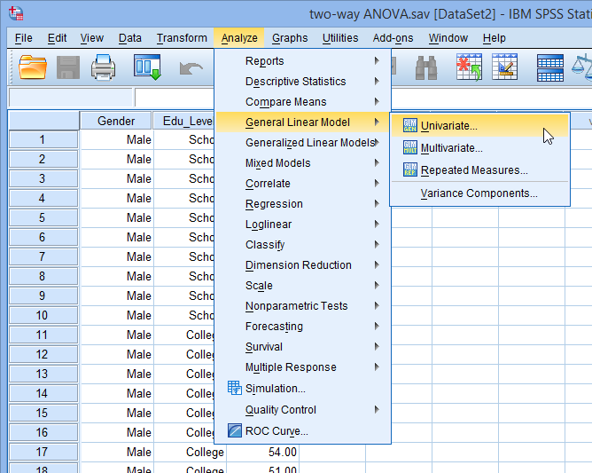
- Click Analyze > General Linear Model > Univariate… on the top menu, as shown below:
Published with written permission from SPSS Statistics, IBM Corporation.
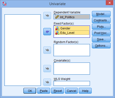
- You will be presented with the Univariate dialogue box, as shown below:

Published with written permission from SPSS Statistics, IBM Corporation.
- Transfer the dependent variable, Int_Politics, into the Dependent Variable: box, and transfer both independent variables, Gender and Edu_Level, into the Fixed Factor(s): box. You can do this by drag-and-dropping the variables into the respective boxes or by using the
 button. If you are using older versions of SPSS Statistics you will need to use the latter method. You will end up with a screen similar to that shown below:
Published with written permission from SPSS Statistics, IBM Corporation.
Note: For this analysis, you will not need to worry about the Random Factor(s):, Covariate(s): or WLS Weight: boxes.
- Click on the
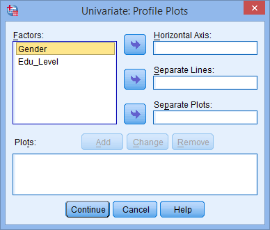
 button. You will be presented with the Univariate: Profile Plots dialogue box, as shown below:
Published with written permission from SPSS Statistics, IBM Corporation.
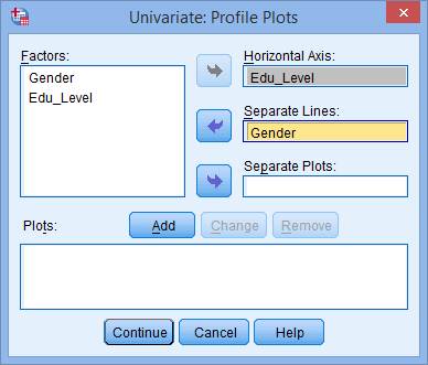
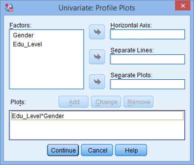
- Transfer the independent variable, Edu_Level, from the Factors: box into the Horizontal Axis: box, and transfer the other independent variable, Gender, into the Separate Lines: box. You will be presented with the following screen:
Published with written permission from SPSS Statistics, IBM Corporation.
Note: It can help to put the independent variable with the greater number of groups in the Horizontal Axis: box.
- Click on the
 button. You will see that “Edu_Level*Gender” has been added to the Plots: box, as shown below:
Published with written permission from SPSS Statistics, IBM Corporation.
- Click on the
 button. This will return you to the Univariate dialogue box.
 - Click on the
 button. You will be presented with the Univariate: Post Hoc Multiple Comparisons for Observed Meansdialogue box, as shown below:
Published with written permission from SPSS Statistics, IBM Corporation.
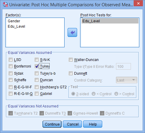
- Transfer Edu_Level from the Factor(s): box to the Post Hoc Tests for: box. This will make the –Equal Variances Assumed– area become active (lose the “grey sheen”) and present you with some choices for which post hoc test to use. For this example, we are going to select Tukey, which is a good, all-round post hoc test.
Note: You only need to transfer independent variables that have more than two groups into the Post Hoc Tests for: box. This is why we do not transfer Gender.
You will finish up with the following screen:
Published with written permission from SPSS Statistics, IBM Corporation.
- Click on the
 button to return to the Univariate dialogue box.
 - Click on the
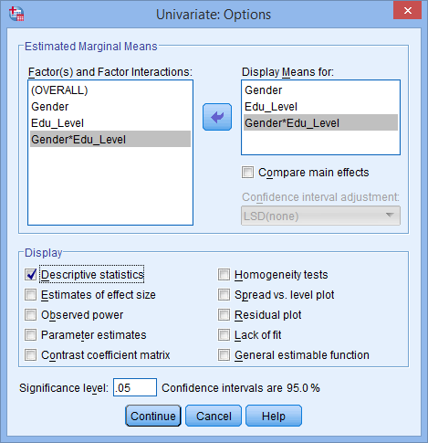
 button. This will present you with the Univariate: Options dialogue box, as shown below:
Published with written permission from SPSS Statistics, IBM Corporation.
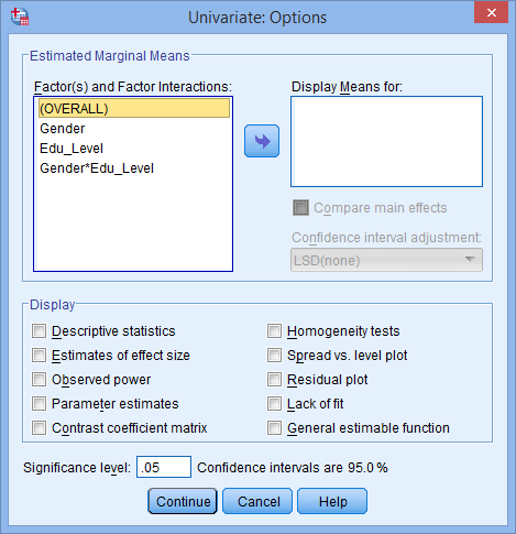
- Transfer Gender, Edu_Level and Gender*Edu_Level from the Factor(s) and Factor Interactions: box into the Display Means for: box. In the –Display– area, tick the Descriptive Statistics option. You will presented with the following screen:
Published with written permission from SPSS Statistics, IBM Corporation.
- Click on the
 button to return to the Univariate dialogue box.
 - Click on the
 button to generate the output.
SPSS Statistics
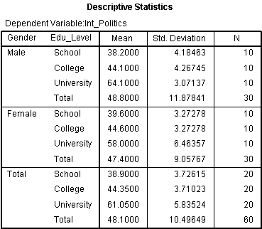
Descriptive statistics
You can find appropriate descriptive statistics for when you report the results of your two-way ANOVA in the aptly named “Descriptive Statistics” table, as shown below:
Published with written permission from SPSS Statistics, IBM Corporation.
This table is very useful because it provides the mean and standard deviation for each combination of the groups of the independent variables (what is sometimes referred to as each “cell” of the design). In addition, the table provides “Total” rows, which allows means and standard deviations for groups only split by one independent variable, or none at all, to be known. This might be more useful if you do not have a statistically significant interaction.
SPSS Statistics
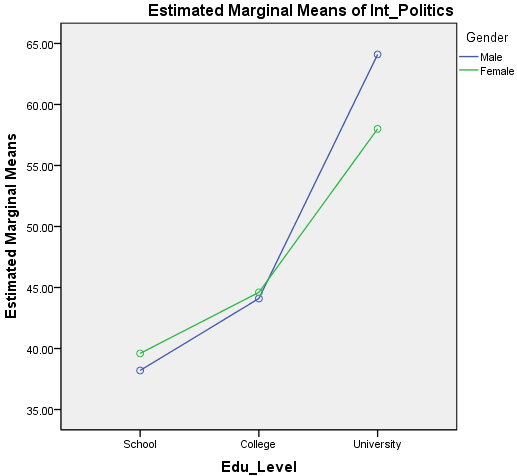
Plot of the results
The plot of the mean “interest in politics” score for each combination of groups of “Gender” and “Edu_level” are plotted in a line graph, as shown below:
Published with written permission from SPSS Statistics, IBM Corporation.
Although this graph is probably not of sufficient quality to present in your reports (you can edit its look in SPSS Statistics), it does tend to provide a good graphical illustration of your results. An interaction effect can usually be seen as a set of non-parallel lines. You can see from this graph that the lines do not appear to be parallel (with the lines actually crossing). You might expect there to be a statistically significant interaction, which we can confirm in the next section.
SPSS Statistics
Statistical significance of the two-way ANOVA
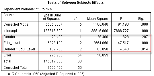
The actual result of the two-way ANOVA – namely, whether either of the two independent variables or their interaction are statistically significant – is shown in the Tests of Between-Subjects Effects table, as shown below:
Published with written permission from SPSS Statistics, IBM Corporation.
The particular rows we are interested in are the “Gender”, “Edu_Level” and “Gender*Edu_Level” rows, and these are highlighted above. These rows inform us whether our independent variables (the “Gender” and “Edu_Level” rows) and their interaction (the “Gender*Edu_Level” row) have a statistically significant effect on the dependent variable, “interest in politics”. It is important to first look at the “Gender*Edu_Level” interaction as this will determine how you can interpret your results (see our enhanced guide for more information). You can see from the “Sig.” column that we have a statistically significant interaction at the p = .014 level. You may also wish to report the results of “Gender” and “Edu_Level”, but again, these need to be interpreted in the context of the interaction result. We can see from the table above that there was no statistically significant difference in mean interest in politics between males and females (p = .207), but there were statistically significant differences between educational levels (p < .0005).
SPSS Statistics
Post hoc tests – simple main effects in SPSS Statistics
When you have a statistically significant interaction, reporting the main effects can be misleading. Therefore, you will need to report the simple main effects. In our example, this would involve determining the mean difference in interest in politics between genders at each educational level, as well as between educational level for each gender. Unfortunately, SPSS Statistics does not allow you to do this using the graphical interface you will be familiar with, but requires you to use syntax. Therefore, in our enhanced two-way ANOVA guide, we show you the procedure for doing this in SPSS Statistics, as well as explaining how to interpret and write up the output from your simple main effects.
When you do not have a statistically significant interaction, we explain two options you have, as well as a procedure you can use in SPSS Statistics to deal with this issue.
SPSS Statistics
Multiple Comparisons Table
If you do not have a statistically significant interaction, you might interpret the Tukey post hoc test results for the different levels of education, which can be found in the Multiple Comparisons table, as shown below:
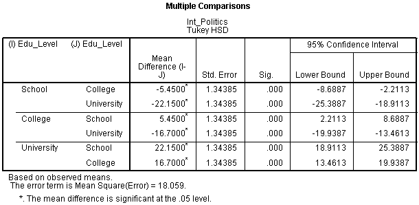
Published with written permission from SPSS Statistics, IBM Corporation.
You can see from the table above that there is some repetition of the results, but regardless of which row we choose to read from, we are interested in the differences between (1) School and College, (2) School and University, and (3) College and University. From the results, we can see that there is a statistically significant difference between all three different educational levels (p < .0005).
SPSS Statistics
Reporting the results of a two-way ANOVA
You should emphasize the results from the interaction first before you mention the main effects. For example, you might report the result as:
- General
A two-way ANOVA was conducted that examined the effect of gender and education level on interest in politics. There was a statistically significant interaction between the effects of gender and education level on interest in politics, F (2, 54) = 4.643, p = .014.
If you had a statistically significant interaction term and carried out the procedure for simple main effects in SPSS Statistics, you would also report these results. Briefly, you might report these as:
- General
Simple main effects analysis showed that males were significantly more interested in politics than females when educated to university level (p = .002), but there were no differences between gender when educated to school (p = .465) or college level (p = .793).