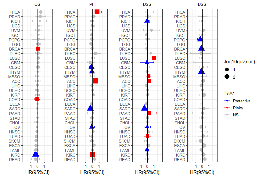
涉及拼图时，有时几个图图例并不完全一样，这时候如何处理，直接上代码（以pancancer生存分析数据为例），此处用到lomon和gridExtra包

library(ggplot2)
setwd("G:/test")
unicox1 <- read.csv("OS_pancan_unicox.csv")
unicox1 <- unicox1[order(unicox1$HR,decreasing = F),]
unicox1$cancer <- factor(unicox1$cancer, levels = unicox1$cancer)
unicox2 <- read.csv("PFI_pancan_unicox.csv")
unicox2$cancer <- factor(unicox1$cancer, levels = unicox1$cancer)
unicox3 <- read.csv("DSS_pancan_unicox.csv")
unicox3$cancer <- factor(unicox1$cancer, levels = unicox1$cancer)
unicox4 <- read.csv("DFI_pancan_unicox.csv")
unicox4$cancer <- factor(unicox1$cancer, levels = unicox1$cancer)

p1 <- ggplot(unicox1, aes(HR,  cancer,  col=Type,shape=Type))+
  geom_point(aes(size=-log10(p.value)))+
  geom_errorbarh(aes(xmax =upper_95, xmin = lower_95), height = 0.4)+
  scale_x_continuous(limits= c(-2, 2), breaks= seq(-1, 1, 1))+
  geom_vline(aes(xintercept = 0))+
  xlab('HR(95%CI)') + ylab(' ')+
  theme_bw(base_size = 12)+
  ggtitle("OS")+
  theme(plot.title = element_text(hjust = 0.5, size=10))+
  scale_color_manual(values = c("gray", "blue", "red"))+theme(legend.position='none')


p2 <- ggplot(unicox2, aes(HR,  cancer,  col=Type,shape=Type))+
  geom_point(aes(size=-log10(p.value)))+
  geom_errorbarh(aes(xmax =upper_95, xmin = lower_95), height = 0.4)+
  scale_x_continuous(limits= c(-2, 2), breaks= seq(-1, 1, 1))+
  geom_vline(aes(xintercept = 0))+
  xlab('HR(95%CI)') + ylab(' ')+
  theme_bw(base_size = 12)+
  ggtitle("PFI")+
  theme(plot.title = element_text(hjust = 0.5, size=10))+guides(shape=FALSE) +
  scale_color_manual(values = c( "blue", "red","gray"),
                     breaks = c("Protective","Risky","NS"),
                     labels = c("Protective","Risky","NS"))+theme(legend.position='none')

p3 <- ggplot(unicox3, aes(HR,  cancer,  col=Type,shape=Type))+
  geom_point(aes(size=-log10(p.value)))+
  geom_errorbarh(aes(xmax =upper_95, xmin = lower_95), height = 0.4)+
  scale_x_continuous(limits= c(-2, 2), breaks= seq(-1, 1, 1))+
  geom_vline(aes(xintercept = 0))+
  xlab('HR(95%CI)') + ylab(' ')+
  theme_bw(base_size = 12)+
  ggtitle("DSS")+
  theme(plot.title = element_text(hjust = 0.5, size=10))+
  scale_color_manual(values = c("gray", "blue", "red"))+theme(legend.position='none')

p4 <- ggplot(unicox4, aes(HR,  cancer,  col=Type,shape=Type))+
  geom_point(aes(size=-log10(p.value)))+
  geom_errorbarh(aes(xmax =upper_95, xmin = lower_95), height = 0.4)+
  scale_x_continuous(limits= c(-2, 2), breaks= seq(-1, 1, 1))+
  geom_vline(aes(xintercept = 0))+
  xlab('HR(95%CI)') + ylab(' ')+
  theme_bw(base_size = 12)+
  ggtitle("DSS")+
  theme(plot.title = element_text(hjust = 0.5, size=10))+
  scale_color_manual(values = c("gray", "blue", "red"))+theme(legend.position='none')

library(gridExtra)
library(lemon)
legend <- g_legend(p2)
grid.arrange(p1, p2,p3,p4,
             ncol = 4, nrow = 1,right=legend)